Reading and processing NIRS data with MNE-Python

This tutorial demonstrates how to read and process NIRS data using MNE-Python and almirah.

Setup

First, we'll import the necessary libraries and set up the logging and warning configurations.

import mne
import warnings
import numpy as np
import matplotlib.pyplot as plt
from itertools import compress

from almirah import Layout

mne.set_log_level(False)
warnings.filterwarnings('ignore')

Loading the Data

Next, we'll set up the layout to access the NIRS data.

lay = Layout(root="/path/to/data", specification_name="bids")
print(lay)

This should output:

<Layout root: '/path/to/data'>

We can query the layout to find all NIRS files with the .snirf extension:

files = lay.query(datatype="nirs", extension=".snirf")
len(files)

This gives the total number of NIRS files:

Querying a Specific File

To query a specific file, we can filter by subject, task, datatype, and extension:

file = lay.query(subject="D0019", task="rest", datatype="nirs", extension=".snirf")[0]
print(file.rel_path)

This should output the relative path of the file:

sub-D0019/ses-111/nirs/sub-D0019_ses-111_task-rest_run-01_nirs.snirf

We can then download the NIRS file:

file.download()

Reading Raw Data

Next, we read the raw NIRS data:

raw = mne.io.read_raw_snirf(file.path)
raw.load_data()

<summary><strong>General</strong></summary>
<table class="table table-hover table-striped table-sm table-responsive small">
    <tr>
        <th>Measurement date</th>
        <td>November 12, 1917  00:00:00 GMT</td>
    </tr>
    <tr>
        <th>Experimenter</th>
        <td>Unknown</td>
    </tr>
    <tr>
        <th>Participant</th>
        <td>mne_anonymize</td>
    </tr>
</table>
</details>
<details open>
    <summary><strong>Channels</strong></summary>
    <table class="table table-hover table-striped table-sm table-responsive small">
        <tr>
            <th>Digitized points</th>
            <td>21 points</td>
        </tr>
        <tr>
            <th>Good channels</th>
            <td>36 fNIRS (CW amplitude)</td>
        </tr>
        <tr>
            <th>Bad channels</th>
            <td>None</td>
        </tr>
        <tr>
            <th>EOG channels</th>
            <td>Not available</td>
        </tr>
        <tr>
            <th>ECG channels</th>
            <td>Not available</td>
        </tr>
    </table>
    </details>
    <details open>
        <summary><strong>Data</strong></summary>
        <table class="table table-hover table-striped table-sm table-responsive small">
            <tr>
                <th>Sampling frequency</th>
                <td>15.62 Hz</td>
            </tr>
            <tr>
                <th>Highpass</th>
                <td>0.00 Hz</td>
            </tr>
            <tr>
                <th>Lowpass</th>
                <td>7.81 Hz</td>
            </tr>
            <tr>
                <th>Filenames</th>
                <td>sub-D0019_ses-111_task-rest_run-01_nirs.snirf</td>
            </tr>
            <tr>
                <th>Duration</th>
                <td>00:10:03 (HH:MM:SS)</td>
            </tr>
        </table>
        </details>

print(raw.info)

<Info | 9 non-empty values
 bads: []
 ch_names: S1_D1 760, S1_D1 850, S1_D2 760, S1_D2 850, S2_D2 760, S2_D2 ...
 chs: 36 fNIRS (CW amplitude)
 custom_ref_applied: False
 dig: 21 items (3 Cardinal, 18 EEG)
 highpass: 0.0 Hz
 lowpass: 7.8 Hz
 meas_date: 1917-11-12 00:00:00 UTC
 nchan: 36
 projs: []
 sfreq: 15.6 Hz
 subject_info: 4 items (dict)
>

Preprocessing

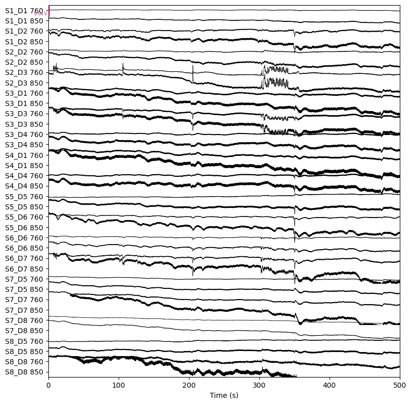
We pick the NIRS channels, compute the source-detector distances, and filter out channels with a distance greater than 0.01:

picks = mne.pick_types(raw.info, meg=False, fnirs=True)
dists = mne.preprocessing.nirs.source_detector_distances(raw.info, picks=picks)
raw.pick(picks[dists > 0.01])
raw.plot(n_channels=len(raw.ch_names), duration=500, show_scrollbars=False)
plt.show()

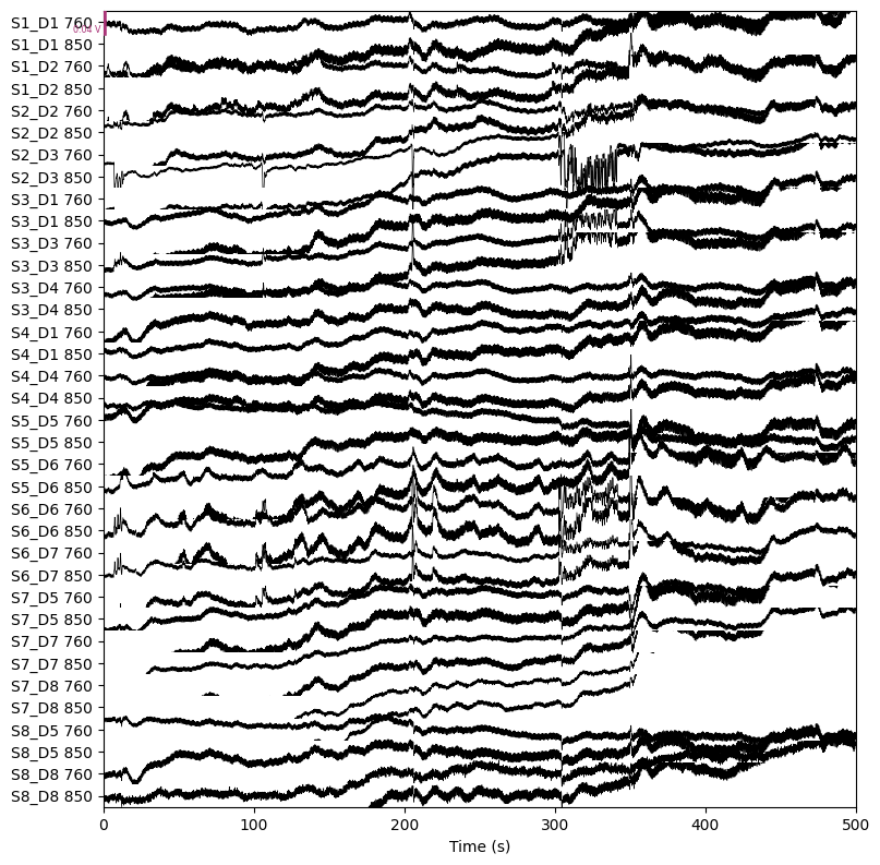
We convert the raw data to optical density:

raw_od = mne.preprocessing.nirs.optical_density(raw)
raw_od.plot(n_channels=len(raw_od.ch_names), duration=500, show_scrollbars=False)
plt.show()

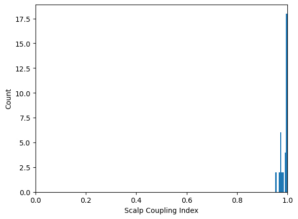
Next, we compute the Scalp Coupling Index (SCI) and plot the distribution:

sci = mne.preprocessing.nirs.scalp_coupling_index(raw_od)
fig, ax = plt.subplots()
ax.hist(sci)
ax.set(xlabel="Scalp Coupling Index", ylabel="Count", xlim=[0, 1])
plt.show()

We mark channels with a low SCI as bad:

raw_od.info["bads"] = list(compress(raw_od.ch_names, sci < 0.5))

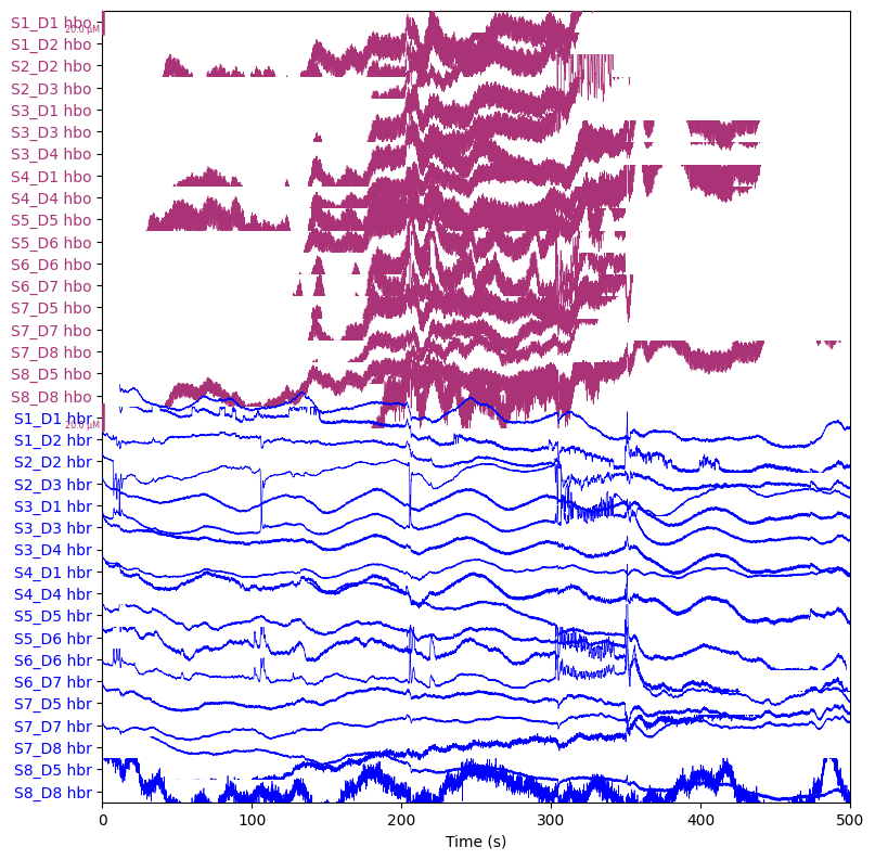
We convert the optical density data to hemoglobin concentration:

raw_haemo = mne.preprocessing.nirs.beer_lambert_law(raw_od, ppf=0.1)
raw_haemo.plot(n_channels=len(raw_haemo.ch_names), duration=500, show_scrollbars=False)
plt.show()

Power Spectral Analysis

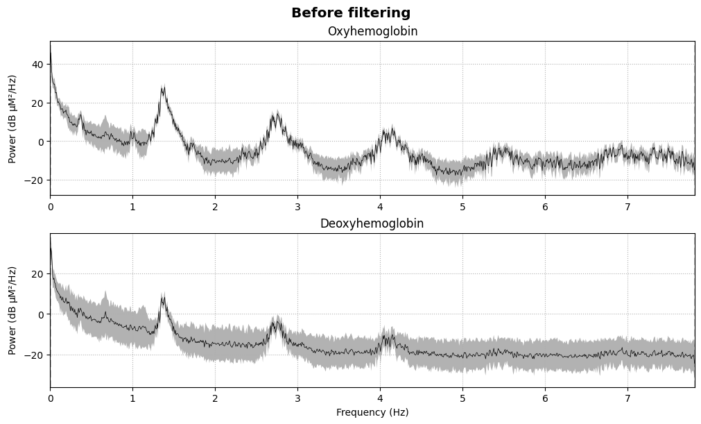
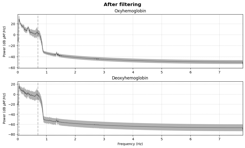
We compute and plot the Power Spectral Density (PSD) before and after filtering:

fig = raw_haemo.compute_psd().plot(average=True, amplitude=False)
fig.suptitle("Before filtering", weight="bold", size="x-large")
raw_haemo = raw_haemo.filter(0.05, 0.7, h_trans_bandwidth=0.2, l_trans_bandwidth=0.02)
fig = raw_haemo.compute_psd().plot(average=True)
fig.suptitle("After filtering", weight="bold", size="x-large")
plt.show()

Epoching

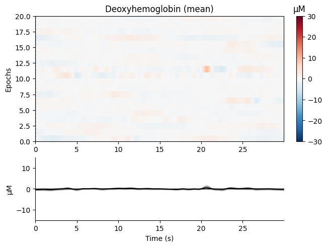
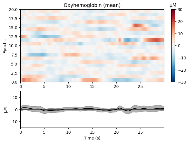
We create epochs from the continuous data:

epochs = mne.make_fixed_length_epochs(raw_haemo, duration=30, preload=False)

Finally, we plot the epochs:

epochs.plot_image(combine="mean", vmin=-30, vmax=30,
                             ts_args=dict(ylim=dict(hbo=[-15, 15],
                                                    hbr=[-15, 15])))
plt.show()

This concludes the tutorial. You've learned how to read, and process near-infrared spectroscopy data using MNE-Python and almirah.

processing-nirs-with-mne.md 6.5 KB Riwayat Download