processing-eeg-with-mne.md 3.9 KB
Processing EEG with MNE-Python
This tutorial demonstrates how to process EEG data using MNE-Python
and almirah. The goal is to show how to interface with other
analysis libraries and generate plots, rather than derive insights.
Setup
First, we'll import the necessary libraries and set up the logging and warning configurations.
import mne
import warnings
import numpy as np
import matplotlib.pyplot as plt

from almirah import Layout

mne.set_log_level(False)
warnings.filterwarnings('ignore')
Loading the Data
Next, we'll set up the layout to access the EEG data.
lay = Layout(root="/path/to/data", specification_name="bids")
lay
This should output:
<Layout root: '/path/to/data'>
We can also get the layout using the specification name:
lay = Layout.get(specification_name='bids')
We can query the layout to find all EEG files with the .vhdr extension:
files = lay.query(datatype="eeg", extension=".vhdr")
len(files)
This gives the total number of EEG files:
2223
Querying Specific Files
To query specific files, we can filter by subject, session, datatype, task, and extension:
vhdr_file = lay.query(subject="D0019", session="101", datatype="eeg", task="rest", extension=".vhdr")[0]
eeg_file = lay.query(subject="D0019", session="101", datatype="eeg", task="rest", extension=".eeg")[0]
montage_file = lay.query(subject="D0019", session="101", space="CapTrak", suffix="electrodes")[0]

print(vhdr_file.rel_path)
This should output the relative path of the file:
sub-D0019/ses-101/eeg/sub-D0019_ses-101_task-rest_run-01_eeg.vhdr
We can then download the EEG file:
eeg_file.download()
Setting Up the Montage and Reading Raw Data
Next, we set up the montage and read the raw EEG data:
montage = mne.channels.read_custom_montage(montage_file.path)
raw = mne.io.read_raw_brainvision(vhdr_file.path, preload=True)
raw.set_montage(montage)
raw.info["bads"] = ["VREF"]

raw.info
General
Measurement date: Unknown
Experimenter: Unknown
Participant: Unknown
Channels
Digitized points: 132 points
Good channels: 128 EEG, 5 misc
Bad channels: VREF
EOG channels: Not available
ECG channels: Not available
Data
Sampling frequency: 1000.00 Hz
Highpass: 0.00 Hz
Lowpass: 500.00 Hz
Preprocessing
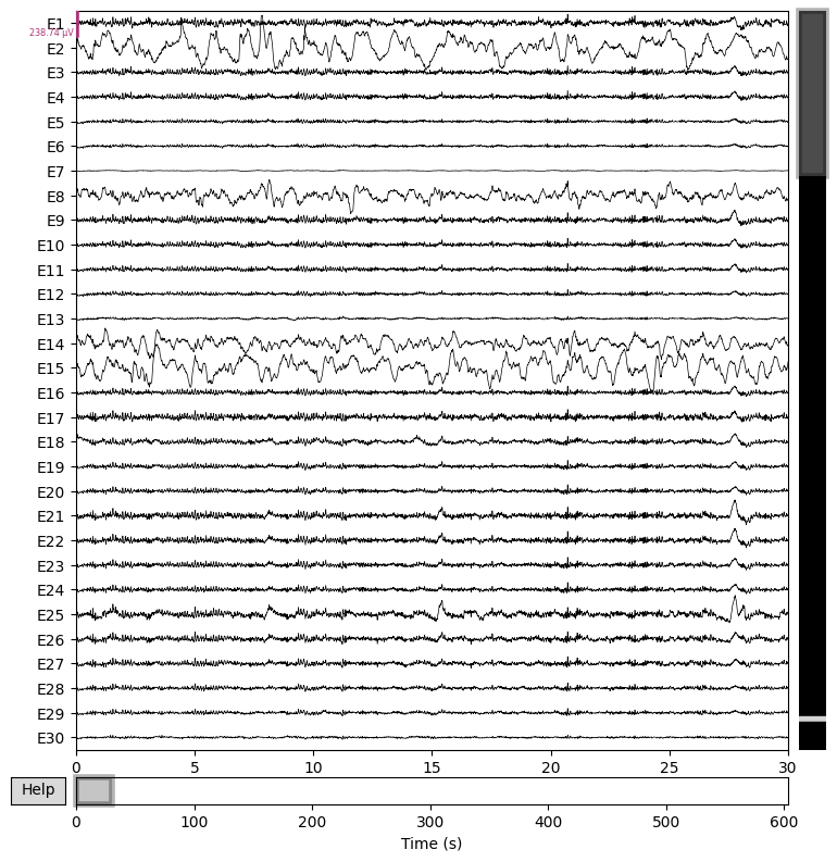
We apply a band-pass filter and plot the raw data:
# Apply a band-pass filter
raw.filter(1, 40, fir_design="firwin")

# Plot the raw data
raw.plot(n_channels=30, duration=30, scalings="auto")
plt.close()
Artifact Removal using ICA
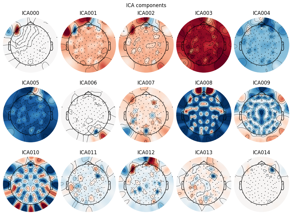
We set up and apply Independent Component Analysis (ICA) to remove artifacts:
# Setup ICA
ica = mne.preprocessing.ICA(n_components=15, random_state=97)
ica.fit(raw)

# Plot ICA components
ica.plot_components()

# Select bad components manually (usually by visual inspection)
ica.exclude = [0, 6, 14]  # Example: components 0 and 1 are eye blinks and heartbeats

# Apply ICA removal
raw_clean = ica.apply(raw.copy())
Power Spectral Analysis
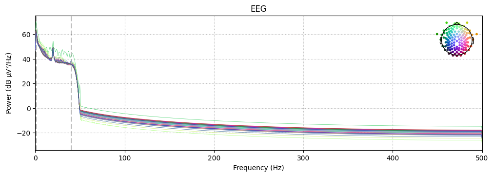
We compute and plot the Power Spectral Density (PSD):
# Compute and plot Power Spectral Density (PSD)
raw_clean.compute_psd().plot(exclude="bads", amplitude=False)
plt.show()
We also plot the topographic distribution of the spectral power:
raw_clean.compute_psd().plot_topomap(ch_type="eeg", agg_fun=np.median)
plt.close()
This concludes the tutorial. You've learned how to interface with
MNE-Python to process EEG data using almirah.


