Average EEG signal across various disorders

This tutorial demonstrates how to compute and visualize the average EEG signal across various disorders using mne, pandas, and seaborn in conjunction with almirah.

Setup

First, we'll import the necessary libraries and set the log level for MNE.

import mne
import pandas as pd
import seaborn as sns

from almirah import Dataset

mne.set_log_level(False)

Loading the Dataset

Next, we'll load the dataset and query the EEG files.

ds = Dataset(name="calm-brain")
eeg_header_files = ds.query(datatype="eeg", task="rest", extension=".vhdr")
eeg_data_files = ds.query(datatype="eeg", task="rest", extension=".eeg")
len(eeg_data_files)

This should give the total number of EEG files:

We then download the EEG data files.

for file in eeg_data_files:
    file.download()

Querying the Database

We connect to the database and query the presenting disorders table.

db = ds.components[2]
db.connect("username", "password")
df = ds.query(table="presenting_disorders")
df[["subject", "session", "addiction"]].head()

This displays the first few rows of the queried table in a DataFrame format.

	subject	session	addiction
0	D0019	101	0
1	D0019	111	0
2	D0020	101	0
3	D0020	111	<NA>
4	D0021	101	0

Processing the EEG Data

We define functions to compute the mean EEG signal and retrieve the disorders.

def get_eeg_mean(file):
    raw = mne.io.read_raw_brainvision(file.path)
    return raw.get_data().mean()

def get_disorders(file):
    disorders = []
    subject, session = file.tags["subject"], file.tags["session"]
    filtered_df = df[(df["subject"] == subject) & (df["session"] == session)]

    if filtered_df.empty:
        print(subject, session)
        return None
    
    for column in ["addiction", "bipolar", "dementia", "ocd", "schizophrenia"]:
        presence = filtered_df.iloc[0][column]
        if not pd.isna(presence) and presence:
            disorders.append(column)
    
    return disorders if disorders else ["healthy"]

def file_func(file):
    mean_eeg, disorders = get_eeg_mean(file), get_disorders(file)

    if not disorders:
        return pd.DataFrame()
        
    mean_df = pd.DataFrame({"mean": [mean_eeg] * len(disorders), "disorder": disorders})
    return mean_df.dropna()

We process the EEG header files to compute the mean EEG signal and retrieve the disorders.

mean_dfs = list(map(file_func, eeg_header_files))
mean_dfs = [df for df in mean_dfs if not df.empty]
mean_df = pd.concat(mean_dfs, sort=False)
mean_df.head()

This displays the first few rows of the combined DataFrame.

	mean	disorder
0	-0.008766	healthy
1	0.000457	addiction
2	-0.006335	healthy
3	-0.002764	healthy
4	-0.008269	ocd

We compute the mean EEG signal for each disorder.

mean_df.groupby("disorder").mean()

This displays the mean EEG signal for each disorder.

	mean
disorder
addiction	0.003414
bipolar	0.001613
dementia	0.010485
healthy	0.002449
ocd	-0.000875
schizophrenia	0.005444

Visualizing the Results

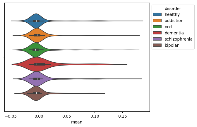
We visualize the distribution of the mean EEG signal for each disorder using a violin plot.

ax = sns.violinplot(data=mean_df, x="mean", hue="disorder")
sns.move_legend(ax, "upper left", bbox_to_anchor=(1, 1))

This generates the plot:

This concludes the tutorial. You've learned how different modalities can be strung together to perform analysis involving multiple modalities.

average-eeg-across-disorders.md 5.7 KB Permalink History Download